Probabilistic Time Series Modeling with Amazon-MxNet-GluonTS
Introduction
Time Series analysis is one of the vital aspects of Artificial Intelligence and Machine Learning. It encompasses activities such as smoothing, forecasting, anomaly detection, etc. A data is often termed as 'time series' if the quantity being measured is varying over time (e.g., currency exchange rate over time, sales over time, energy usage over time, etc.). Given a time-varying quantity, predicting its path over the future has been around for a while. Many standard machine learning libraries have been offering solutions to address the 'point-estimate' of time series in the future horizon. However, nowadays there is a growing trend among businesses that they are often faced with questions like the following ones from their customers:
- How confident are you with your model?
- What extend (in terms of some business metrics) can we trust your model?
- What is the expected deviation of the forecast that your model is providing?
It becomes rather difficult to address these questions with the so called 'point-estimate' time series forecasting. Thus there is a growing research around finding explanations for the way machine learning models get to behave. Probabilistic time series modeling is one of the ways of addressing this challenge. In this respect, AWS open-sourced its Apache MxNet-based toolkit, GluonTS, for probabilistic time series analysis last year. GluonTS incorporates various deep-learning-based probabilistic time series modeling approaches both from AWS and the literature. In this article, I will demonstrate how we can very easily build a probabilistic time series model using GluonTS, and will discuss some of its salient features.
GitHub
You can find a working copy of a python script in my personal GitHub repository so that you can give a try for yourself right away.
Dataset
As far as the dataset is concerned in GluonTS, we have three following choices:
- Use an in-build time series dataset available in GluonTS
- Create an artificial time series dataset with GluonTS
- Adapt any external time series dataset for GluonTS
GluonTS comes with a handful of in-build time series datasets covering various sectors such as finance, energy, public, etc. An artificial data (the term 'data' refers to time series data from now onwards throughout this article) can be generated using the synthetic data generation tool of GluonTS. Any external data can be converted into a dataset recognized by GluonTS using its ListDataset class. For an example:
# get the csv file as a dataframe
raw_data = pd.read_csv("https://raw.githubusercontent.com/numenta/NAB/master/data/realTweets/Twitter_volume_AMZN.csv",header=0,index_col=0)

# convert the raw data into an object recognised by GluonTS
# start: the starting index of the dataframe
# target: the actual time series data that we want to model
# freq: the frequency with which the data is collected
train_data = common.ListDataset([{"start": raw_data.index[0], "target": raw_data.value[:"2015-04-05 00:00:00"]}], freq="5min")
I am going to use the exchange_rate dataset available in GluonTS for the purpose of demonstration. An in-build dataset has 3 main members: train, test & metadata. As the name suggests, the 'train' member has the training data. The 'test' member has both the training & the test data (an additional last window of the time series which is of length equal to 'prediction length' or 'forecast horizon' as it is known in time series modeling). The 'metadata' member has various information about the dataset (e.g., the frequency of the data collected, prediction length, features, etc.). The data can further be transformed or new features can be generated using the 'Transformation' feature of GluonTS. However, we will not exercise it for the sake of simplicity. The 'train' dataset is shown below.
# get the financial data "exchange_rate"
gluon_data = get_dataset("exchange_rate", regenerate=True)
train_data = next(iter(gluon_data.train))
test_data = next(iter(gluon_data.test))
meta_data = gluon_data.metadata

# visualize various members of the 'gluon_data.*'
print(train_data.keys())
print(test_data.keys())
print(meta_data)
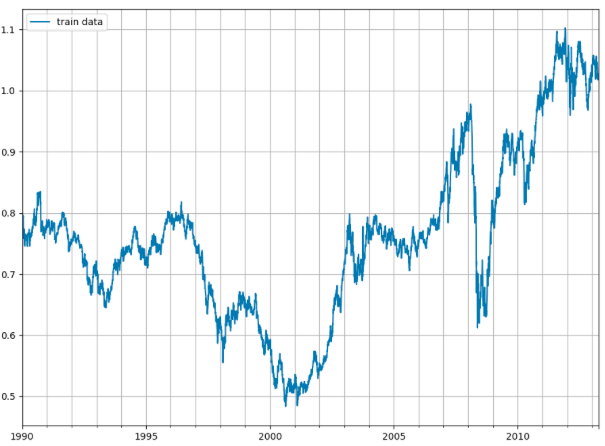
Training dataset
Modeling
GluonTS comes with a variety of probabilistic time series modeling approaches. The available models can be observed here . We will choose DeepAR approach as it is also used to power the Amazon Forecast service offered by AWS (optionally refer to my article on Amazon Forecast). However, it is mentioned that the implementation of DeepAR in GluonTS is not related to the one that is used in Amazon Forecast.
GluonTS uses slightly different modeling conventions which may be confusing at first. A model before training is denoted as an 'Estimator'. The 'Estimator' object, however, represents details about the model such as coefficients, weights, etc. Estimator is configured by 'Trainer' object that defines how (e.g., usage of GPU/CPU, batch size, number of epochs, learning rate, etc.) the Estimator should be trained. The Estimator can be further trained with training data (i.e., the 'train' member of the dataset). The trained model is known as 'Predictor'. As expected, 'Predictor' is the one that will be used to get forecasts. The Predictor can further be serialised/deserialised (i.e., saved/loaded) using its member functions 'serialize & deserialize'. For an example:
# create an Estimator with DeepAR
# an object of Trainer() class is used to customize Estimator
estimator = deepar.DeepAREstimator(freq=meta_data.freq, prediction_length=meta_data.prediction_length, trainer=Trainer(ctx="cpu", epochs=200, learning_rate=1e-4))

# create a Predictor by training the Estimator with training dataset
predictor = estimator.train(training_data=training_data)

# save the Predictor
predictor.serialize(Path("/folder_name/"))
If we have to include (time series) features during model building, these features have to be included in the 'train' & 'test' members of the dataset, and the corresponding parameters (e.g., 'use_feat_dynamic_real = True' in case of DeepAREstimator ) should be set appropriately. More information on this can be obtained here (the official documentation). It is important to note that many time series datasets (not just features) can be included to build a single model.
Forecasting
Forecasts can be constructed as simple as shown below.
# make predictions
forecasts, ts_it = make_evaluation_predictions(dataset=testing_data, predictor=predictor, num_samples=200)
Forecasts are made for the complete 'forecast horizon' as it was mentioned during the configuration of the 'Estimator'. The model accuracy is reasonably good for the first attempt, however can be improved by paying more attention to the model hyper-parameters.
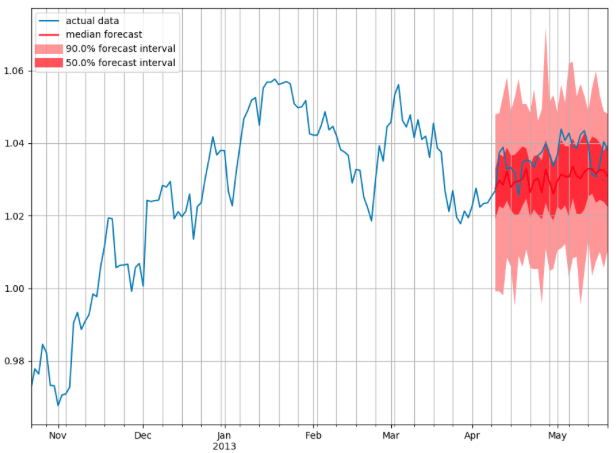
Forecasts
One of the interesting features of GluonTS is to perform backtesting on its own in order to provide various performance metrics. There is no need to implement (of course, possible if needed) any of the error metrics as most of them are already available in GluonTS. This eradicates the usual uncertainty over the bug-less implementation of various error metrics to make a feasible comparison across various models. We can create our own models using GluonTS too as it provides various founding blocks of the model building and evaluation. However, it is worth writing a separate article on that, thus we will stop here for the sake of simplicity.
Highlights
It is definitely an interesting and a very useful deep-learning (time series) library for experimentation. One can create a significant amount of variations of the existing state-of-the-art probabilistic (neural) time series models. As it is geared towards research experimentation, it has simplified various aspects of model building and testing as stated earlier. For an example, it has a very simple way of comparing GluonTS's models and their variations with Facebook's Prophet time series package. However, there is not much information over how the model built using GluonTS can be taken to production. I guess we can make use of MxNet Multi Model Server or Amazon SageMaker . I will probably write more about this in the coming months.